Low cross-taxon congruence and weak stand-age effects on biodiversity in Swedish oak forests
Six taxonomic groups. Twenty-five oak stands aged 19 to 165 years. 22,276 taxa. Almost none of it lines up the way forest conservation has long assumed.
The same study, re-verified from the deposited data and wired to the global species web
Every figure below was recomputed from the authors’ own Figshare matrices rather than transcribed from the PDF, and every one of the 368 named lichens, bryophytes and vascular plants has been re-matched to the current GBIF Backbone Taxonomy, cross-linked to iNaturalist, and screened against the IUCN Red List 2026-1. No national checklist is used anywhere, so every species here is addressable from anywhere in the world.
The finding, in one paragraph
Conservation planning leans hard on two shortcuts: that a well-surveyed indicator group stands in for biodiversity at large, and that older forest holds more of it. Across 25 production oak stands in southern Sweden, neither shortcut survives contact with the data. Species richness in insects, arachnids, springtails, epiphytic lichens, bryophytes and vascular plants was measured in the same stands — and not one of the 15 possible pairs of groups was correlated (r from -0.28 to +0.34, smallest p = 0.092). Only lichens grew richer with stand age. Springtails peaked in middle-aged stands. The remaining four groups — 98% of all taxa recorded — were flat.
Composition told a gentler version of the same story: stand age shifted which species were present in four groups, but explained under 10% of the variation in all of them except lichens (17%). Geography mattered at least as much as age nearly everywhere.
Richness by group
| Group | Total taxa | Mean/stand | SE | Min | Max | Share | Unit |
|---|---|---|---|---|---|---|---|
| Insects | 20,630 | 3828.6 | 127.1 | 2,933 | 5,297 | 92.6% | COI OTUs |
| Arachnids | 962 | 158.9 | 4.9 | 120 | 199 | 4.3% | COI OTUs |
| Springtails | 316 | 71.8 | 3.2 | 45 | 114 | 1.4% | COI OTUs |
| Lichens | 167 | 34.1 | 1.9 | 21 | 63 | 0.7% | named species |
| Bryophytes | 46 | 9.8 | 0.8 | 2 | 17 | 0.2% | named species |
| Vascular plants | 155 | 24.7 | 2.0 | 6 | 46 | 0.7% | named species |
| All groups | 22,276 | 4128 | 127.6 | 3,267 | 5,597 | 100% |
Arthropods were identified as COI metabarcoding OTUs clustered at 97% similarity, so their counts are operational taxa rather than named species. Lichens, bryophytes and vascular plants were identified in the field to species and are the 368 taxa carried through the species explorer below.
Everything checked, twice — six clean reproductions and two things worth fixing
The published analysis was re-run from scratch in Python (negative-binomial GLMs, Pearson congruence, Bray–Curtis NMDS, and a from-first-principles McArdle–Anderson PERMANOVA) against the deposited matrices. The statistical substance holds up completely. Two bookkeeping errors surfaced, neither of which changes a conclusion.
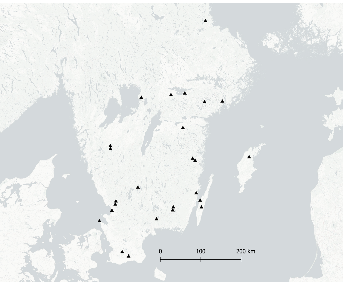
Twenty-five oak stands, 19 to 165 years old, across southern Sweden
Stands were selected in 2022 to span the widest age range available in production forestry, deliberately excluding pre-canopy-closure stands (<15 yr) and truly ancient ones (>200 yr). Age is the mean of increment cores from ten dominant Quercus robur per stand, cross-dated with COFECHA. Circle size shows stand area; fill shows age. Click any stand.
Stand explorer
| Stand ▼ | Age (yr) ▼ | Size (ha) ▼ | Lat °N ▼ | Lon °E ▼ | Soil | Insects ▼ | Arachnids ▼ | Springtails ▼ | Lichens ▼ | Bryophytes ▼ | Vascular ▼ | Total ▼ | Age |
|---|
No group predicts any other group
Fifteen pairwise Pearson correlations of stand-level richness. None is statistically significant; the strongest relationship in the entire matrix (insects × vascular plants, r = +0.34) would still leave 88% of the variation unexplained. Click any cell to see the raw scatter.
Stand age moves lichens, bends springtails, and leaves everything else alone
Negative-binomial GLMs of richness against stand age (linear and quadratic), latitude, longitude and — for the Malaise-trapped arthropods — trapping days. Curves are model predictions with 95% confidence bands; points are the 25 stands. Hover a point for its stand, click to open it.
All coefficients at a glance
Standardised effects on the log scale, so magnitudes are comparable across groups. Filled circles are significant at p < 0.05.
Coefficient table — reproduction against Table S2
| Group | Intercept | Trapping days | Stand age | Stand age² | Latitude | Longitude |
|---|---|---|---|---|---|---|
| Insects | +8.247 (0.027) * p=<0.001 +8.250 | -0.026 (0.031) p=0.401 -0.025 | — | — | +0.076 (0.031) * p=0.015 +0.075 | +0.004 (0.034) p=0.916 +0.005 |
| Arachnids | +5.066 (0.027) * p=<0.001 +5.070 | +0.046 (0.031) p=0.141 +0.046 | — | — | -0.022 (0.031) p=0.474 -0.023 | -0.027 (0.035) p=0.440 -0.026 |
| Springtails | +4.259 (0.027) * p=<0.001 +4.260 | +0.045 (0.035) p=0.200 +0.043 | +0.432 (0.111) * p=<0.001 +0.430 | -0.356 (0.112) * p=0.002 -0.358 | -0.053 (0.034) p=0.115 -0.052 | -0.071 (0.036) * p=0.048 -0.075 |
| Lichens | +3.521 (0.046) * p=<0.001 +3.520 | — | +0.107 (0.049) * p=0.028 +0.106 | — | -0.033 (0.054) p=0.542 -0.029 | +0.077 (0.052) p=0.136 +0.073 |
| Bryophytes | +2.275 (0.079) * p=<0.001 +2.270 | — | — | — | +0.073 (0.088) p=0.409 +0.071 | +0.024 (0.090) p=0.789 +0.027 |
| Vascular plants | +3.177 (0.065) * p=<0.001 +3.180 | — | — | — | +0.179 (0.073) * p=0.014 +0.179 | +0.114 (0.074) p=0.125 +0.115 |
Each cell: refitted standardised estimate (SE), p-value, and in grey the published value from Table S2 after correcting the transposed Latitude/Longitude headers (see Corrections). * marks p < 0.05. Stand size had no relationship with any group and was excluded from all published models.
A sensitivity check the paper did not run
If a quadratic age term is forced into every model, how much support does it attract? Only springtails show a strong unimodal signal — but vascular plants come surprisingly close, with a hump-shaped fit that is essentially tied with the published model on AIC.
| Group | Age in published model | Age β | p | Age² β | p | ΔAIC |
|---|---|---|---|---|---|---|
| Insects | — | +0.030 | 0.776 | -0.037 | 0.733 | +3.86 |
| Arachnids | — | +0.099 | 0.336 | -0.136 | 0.198 | +1.61 |
| Springtails | in model | +0.432 | <0.001 | -0.356 | 0.002 | +0.00 |
| Lichens | in model | +0.054 | 0.763 | +0.055 | 0.755 | +1.91 |
| Bryophytes | — | +0.337 | 0.270 | -0.263 | 0.383 | +2.38 |
| Vascular plants | — | +0.393 | 0.098 | -0.464 | 0.053 | +0.04 |
Which species are present shifts with age — but only a little, and mostly for lichens
Non-metric multidimensional scaling on Bray–Curtis dissimilarities, with marginal PERMANOVA on stand age, latitude and longitude. Points are stands, filled by age: if age structured composition strongly, light and dark points would separate cleanly. Toggle the Shepard diagrams to judge how faithfully each 2- or 3-dimensional picture represents the real dissimilarities.
PERMANOVA — reproduction against Table S3
| Group | Stand age | Latitude | Longitude | Residual R² | ||||||
|---|---|---|---|---|---|---|---|---|---|---|
| R² | p | published | R² | p | published | R² | p | published | ||
Table 1. Marginal (type-III) distance-based pseudo-F, 1999 permutations, computed here from the full three-term model for every group; grey columns give the published R²/p from Table S3, where each group was tested in its own reduced final model. Agreement is close throughout — including for bryophytes, whose significant age effect is missing from the paper’s Results text.
All 368 named species — every one linked, re-named and Red-Listed
The 167 lichens, 46 bryophytes and 155 vascular plants identified in the field, resolved against the current GBIF Backbone, matched to iNaturalist (368 of 368), screened against IUCN Red List 2026-1, and joined to what the study data say about where each one actually grew. Search, filter, sort, click any row for the full record — or export the whole filtered set.
| Species ▼ | Family ▼ | IUCN ▼ | Stands ▼ | Records ▼ | Mean age ▼ | Age affinity ▼ | GBIF recs ▼ | iNat obs ▼ | Links |
|---|
What “records” counts
Lichens and bryophytes were surveyed on the trunks of the same ten oaks per stand, ground level to 2 m, so a species can score 1–10 per stand. Vascular plants were recorded in forty 0.5 m² plots per stand (1–40), excluding grasses and sedges. Totals are summed across all 25 stands.
What “age affinity” means
A new metric, not in the paper: the mean age of the stands a species occupies, expressed as standard deviations from the mean age of all 25 stands (83.0 yr). Positive means the species tilts old, negative means it tilts young. It is descriptive — with 25 stands it flags candidates, it does not test them.
Why no Dyntaxa or Artfakta
Sweden’s national taxonomic and Red List services are excellent but national. Resolving every name through the GBIF Backbone and linking to iNaturalist means a reader in Osaka or Oaxaca can open the same species page, see the same accepted name, and pull the same occurrence records.
Which families carry the diversity
The eighteen richest families among the named taxa. Click any bar to filter the explorer to that family.
Fewest records worldwide
The ten taxa in this study with the smallest global GBIF footprint. Read it as a recording-effort ranking rather than a rarity ranking — obscure crustose lichens are under-recorded everywhere — but it is a useful shortlist of what these stands hold that few datasets do.
| Taxon | GBIF world | Sweden | Stands | IUCN |
|---|
The unnamed 21,908
Honesty about what cannot be linked: the arthropods in this study exist as COI sequence clusters, not as names. An OTU assigned only to a family or order has no species page anywhere — which is precisely why these three groups contribute 98.3% of the taxa and 0% of the species links. Their group-level pages are below; the sequences themselves live with the paper’s Figshare deposit.
Insects — 20,630 OTUs
93% of everything recorded, and the group with no age signal at all.
Arachnids — 962 OTUs
Under-sampled by design: a Malaise trap catches poorly for ground-dwelling spiders, as the authors note.
Springtails — 316 OTUs
The one group with a hump-shaped age response, peaking in middle-aged stands.
43 of 368 names have moved since the paper went to press
32 published names are now synonyms under the current GBIF Backbone — the lichen genera have been especially busy — and the rest are orthographic corrections or aggregate labels resolved to an accepted taxon. Nothing here is an error in the original paper: this is what four years of active systematics does to a species list. Names in the species explorer above are the current ones, with the published name shown struck through.
| Group | As published (2025) | Current accepted name | Why it changed | Type | GBIF |
|---|---|---|---|---|---|
| Bryophytes | rhytidiadelphus triquetrus | Hylocomiadelphus triquetrus (Hedw.) Ochyra & Stebel | published name is a synonym in the current backbone | synonym | G |
| Bryophytes | orthothricum speciosum | Lewinskya speciosa (Nees) F.Lara, Garilleti & Goffinet | published name is a synonym in the current backbone | synonym | G |
| Bryophytes | orthothricum striatum | Lewinskya striata (Hedw.) F.Lara, Garilleti & Goffinet | published name is a synonym in the current backbone | synonym | G |
| Bryophytes | dicranum montanum | Orthodicranum montanum (Hedw.) Loeske | published name is a synonym in the current backbone | synonym | G |
| Lichens | arthonia ruana | Arthothelium ruanum (A.Massal.) Körb. | published name is a synonym in the current backbone | synonym | G |
| Lichens | mycobilimbia epixanthoides | Biatora epixanthoides (Nyl.) Diederich | published name is a synonym in the current backbone | synonym | G |
| Lichens | caloplaca ulcerosa | Coppinsiella ulcerosa (Coppins & P.James) S.Y.Kondr. & Lőkös | published name is a synonym in the current backbone | synonym | G |
| Lichens | arthonia spadicea | Diarthonis spadicea (Leight.) Frisch, Ertz, Coppins & P.F.Cannon | published name is a synonym in the current backbone | synonym | G |
| Lichens | lecanora carpinea leptyrodes | Glaucomaria carpinea (L.) S.Y.Kondr., Lőkös & Farkas | published name is a synonym in the current backbone | synonym | G |
| Lichens | biatora ocelliformis | Ivanpisutia ocelliformis (Nyl.) S.Y.Kondr. | published name is a synonym in the current backbone | synonym | G |
| Lichens | caloplaca lucifuga | Lendemeriella lucifuga (G.Thor) S.Y.Kondr. | published name is a synonym in the current backbone | synonym | G |
| Lichens | pertusaria albescens | Lepra albescens (Huds.) Hafellner | published name is a heterotypic synonym in the current backbone | synonym | G |
| Lichens | arthonia cinereopruinosa | Leprantha cinereopruinosa (Schaer.) Körb. | published name is a synonym in the current backbone | synonym | G |
| Lichens | arthopyrenia punctiformis | Naetrocymbe punctiformis (Pers.) R.C.Harris | published name is a synonym in the current backbone | synonym | G |
| Lichens | tuckermannopsis chlorophylla | Nephromopsis chlorophylla (Willd.) Divakar, A.Crespo & Lumbsch | published name is a synonym in the current backbone | synonym | G |
| Lichens | gyalolechia flavorubescens | Opeltia flavorubescens (Huds.) S.Y.Kondr. & Hur | published name is a synonym in the current backbone | synonym | G |
| Lichens | gyalecta fagicola | Pachyphiale fagicola (Arnold) Zwackh | published name is a synonym in the current backbone | synonym | G |
| Lichens | lepra borealis pertusaria pupillaris | Pertusaria borealis Erichsen | published name is a synonym in the current backbone | synonym | G |
| Lichens | physcia endophoenicea | Phaeophyscia endophoenicea (Harm.) Moberg | published name is a synonym in the current backbone | synonym | G |
| Lichens | myriolecis hagenii | Polyozosia hagenii (Ach.) S.Y.Kondr., Lőkös & Farkas | published name is a synonym in the current backbone | synonym | G |
| Lichens | porina leptalea | Segestria leptalea (Durieu & Mont.) R.C.Harris | published name is a synonym in the current backbone | synonym | G |
| Lichens | lecanora varia | Straminella varia (Hoffm.) S.Y.Kondr., Lőkös & Farkas | published name is a synonym in the current backbone | synonym | G |
| Lichens | strigula jamesii | Swinscowia jamesii (Swinscow) S.H.Jiang, Lücking & Sérus. | published name is a synonym in the current backbone | synonym | G |
| Vascular plants | Epilobium angustifolium | Chamaenerion angustifolium (L.) Scop. | published name is a heterotypic synonym in the current backbone | synonym | G |
| Vascular plants | Trientalis europaea | Lysimachia europaea (L.) U.Manns & Anderb. | published name is a heterotypic synonym in the current backbone | synonym | G |
| Vascular plants | Cicerbita muralis | Mycelis muralis (L.) Dumort. | published name is a homotypic synonym in the current backbone | synonym | G |
| Vascular plants | Stellaria holostea | Rabelera holostea (L.) M.T.Sharples & E.A.Tripp | published name is a synonym in the current backbone | synonym | G |
| Vascular plants | Rubus nessensis | Rubus polonicus Barr. ex Weston | published name is a synonym in the current backbone | synonym | G |
| Vascular plants | Sorbus intermedia | Scandosorbus intermedia (Ehrh.) Sennikov | published name is a synonym in the current backbone | synonym | G |
| Vascular plants | Lycopodium annotinum | Spinulum annotinum (L.) A.Haines | published name is a synonym in the current backbone | synonym | G |
| Vascular plants | Myosoton aquaticum | Stellaria aquatica (L.) Scop. | published name is a synonym in the current backbone | synonym | G |
| Vascular plants | Taraxacum sect Taraxacum | Taraxacum officinale Weber ex F.H.Wigg. | published name is a synonym in the current backbone | synonym | G |
| Bryophytes | eurynchium striatum | Eurhynchium striatum (Schreb. ex Hedw.) Schimp. | orthographic correction | spelling | G |
| Bryophytes | fissidens adanthoides | Fissidens Hedw. | orthographic correction | spelling | G |
| Bryophytes | frullania fragillifolia | Frullania fragilifolia (Taylor) Gottsche, Lindenb. & Nees | orthographic correction | spelling | G |
| Bryophytes | porella cordeana | Porella cordaeana (Huebener) Moore | orthographic correction | spelling | G |
| Lichens | bryostigma muscigena | Bryostigma muscigenum (Th.Fr.) Frisch & G.Thor | orthographic correction | spelling | G |
| Lichens | chaenotheca chrycocephala | Chaenotheca chrysocephala (Ach.) Th.Fr. | orthographic correction | spelling | G |
| Lichens | haemmatomma ochroleuchum | Haematomma ochroleucum (Neck.) J.R.Laundon | orthographic correction | spelling | G |
| Lichens | hypocenemyce scalaris | Hypocenomyce scalaris (Ach.) M.Choisy | orthographic correction | spelling | G |
| Lichens | lecidella rinodina sp sorediose | Lecidella Körb., 1855 | aggregate/uncertain label resolved to the accepted taxon | spelling | G |
| Lichens | opegrapha vermicillifera | Opegrapha vermicellifera (J.Kunze) J.R.Laundon | orthographic correction | spelling | G |
| Lichens | parmeliella triptophylla | Parmeliella thriptophylla (Ach.) Müll.Arg. | orthographic correction | spelling | G |
Which species actually lean old, and which lean young
The paper tests groups; this tests species. For every taxon found in at least three stands, the mean age of its occupied stands is compared with the mean of all 25. The twelve strongest tilts in each direction are shown. Click any bar for the species record.
Species × stand, with stands ordered youngest to oldest
The full field-survey matrix. Colour intensity is the number of trees (or plots) occupied. Reading left to right is reading up the age gradient — the lichen panel is the only one where the occupied cells visibly drift rightwards.
Column headers give stand code and stand age in years. Click a species name or cell to open the species record.
318 of 368 species have never been assessed globally
Screening the full named list against IUCN Red List 2026-1 produces a stark asymmetry: nearly every vascular plant has a global assessment, and almost no lichen or bryophyte does. That is not a gap in this dataset — it is the state of global assessment for these groups, and it is the reason a study like this one cannot lean on Red List categories to judge a stand’s value.
The two that stand out
Fraxinus excelsior — common ash — is listed NT Near Threatened globally, driven by ash dieback (Hymenoscyphus fraxineus) across its European range. It was recorded in the understory of these oak stands, which makes them incidental refugia for a declining tree.
Malus sylvestris — European crab apple — is DD Data Deficient: its status is genuinely unknown because hybridisation with cultivated apple makes wild populations hard to delimit.
Why so many blanks
Global Red List coverage is concentrated in vertebrates and vascular plants. Lichens and bryophytes have been assessed only in scattered national and regional efforts, so a globally NE lichen may still be red-listed nationally — including in Sweden. The signal to take from this panel is not that these species are safe; it is that no global instrument currently says anything about them.
Two things to fix in the record
Both were found by recomputing rather than by reading, and both are labelling rather than analysis. Neither changes an estimate, a p-value or a conclusion. They are recorded here because a reader using Table S2 or the Results text at face value would draw a wrong inference about geography.
1. Table S2: the Latitude and Longitude columns are transposed
Refitting each published model gives coefficients that match Table S2 only if the two geographic columns are exchanged. The pattern is consistent across all 5 rows that contain both terms, and the mismatch is not marginal: as labelled the values disagree by 0.117 on average, swapped they agree to 0.004.
| Group | Refit latitude β | Refit longitude β | Table S2 “Latitude” | Table S2 “Longitude” | Error as labelled | Error if swapped | Verdict |
|---|---|---|---|---|---|---|---|
| Insects | +0.076 | +0.004 | +0.005 | +0.075 | 0.142 | 0.002 | swapped |
| Arachnids | -0.022 | -0.027 | -0.026 | -0.023 | 0.008 | 0.002 | swapped |
| Lichens | -0.033 | +0.077 | +0.073 | -0.029 | 0.212 | 0.008 | swapped |
| Bryophytes | +0.073 | +0.024 | +0.027 | +0.071 | 0.093 | 0.005 | swapped |
| Vascular plants | +0.179 | +0.114 | +0.115 | +0.179 | 0.129 | 0.001 | swapped |
Likely mechanism. In Final_code.R every model is written … + x_sweref99 + y_sweref99, i.e. easting (longitude) before northing (latitude) — and the script itself defines Long = x_sweref99; Lat = y_sweref99 when plotting. Table S2’s headers run Latitude then Longitude, so coefficients pasted in formula order land under the opposite labels.
What actually changes. The significant geographic effects are real but point the other way than the table implies: insect richness rises towards the north (not east), vascular plant richness rises towards the north, and the springtail geographic effect is longitudinal. Table S3 (PERMANOVA) is not affected — its labels check out against this reproduction, because there the lichen and plant final models retained only x_sweref99 and it appears correctly as Longitude.
2. Results text: bryophytes, not arachnids
The Results section reads: “Stand age significantly affected species composition for arachnids, springtails, lichens, and vascular plants, but not for insects.” Table S3 lists stand age as significant for Collembola, Lichens, Bryophytes and Vascular plants — arachnids do not appear. This reproduction agrees with the table:
- Bryophytes — stand age R² = 0.098, p = 0.014 (significant); Table S3 gives R² = 0.10, p = 0.012.
- Arachnids — stand age R² = 0.050, p = 0.073 (not significant); stand age was dropped from the arachnid final model.
The sentence should name bryophytes. The paper’s argument is untouched — four of six groups still show a compositional shift with age, and the explanatory power is still under 10% everywhere except lichens.
How this edition was built
Sources
- Paper: Johansson V, Forsman A, Gustafsson L, Hall M, Edvardsson J, Salis R, Sunde J, Franzén M (2025) Low cross-taxon congruence and weak stand-age effects on biodiversity in Swedish oak forests. Biodiversity and Conservation 34:2739–2750. doi:10.1007/s10531-025-03093-y (CC BY 4.0)
- Data and code: the authors’ Figshare deposit doi:10.6084/m9.figshare.27100996 — six site × taxon matrices, stand-level covariates, and Final_code.R.
- Supplementary Appendix S1: Tables S1–S3 and Fig S1, parsed directly from the published .docx.
- Taxonomy: GBIF Backbone Taxonomy (checklistbank nub), queried 2026-08-05, via the GBIF species match and search APIs.
- Conservation status: IUCN Red List 2026-1 (released 9 July 2026, 175,909 species assessed), read through GBIF’s Red List mirror.
- Links, common names, photographs: the iNaturalist API. 296 taxa carry an openly licensed photograph (CC0 / CC BY / CC BY-NC / CC BY-SA and variants); every photograph keeps its photographer credit and licence in the species record.
- Basemap: country outlines from the open geo-countries dataset, clipped to the study window and simplified with Ramer–Douglas–Peucker.
What was recomputed, and how
- Richness and totals — rebuilt from the presence/absence structure of each matrix and checked against the authors’ own richness columns (150/150 values identical).
- Congruence — 15 Pearson correlations of stand-level richness, scipy.stats.
- GLMs — negative binomial with log link, dispersion by profile likelihood, statsmodels; predictors z-standardised as in the paper. Both the published model structures and an exhaustive AIC search over all term subsets were fitted.
- Ordination — Bray–Curtis dissimilarities; Kruskal non-metric MDS implemented from scratch (isotonic regression alternated with L-BFGS descent on stress-1), 31 starts per group, rotated to principal axes.
- PERMANOVA — McArdle & Anderson (2001) distance-based pseudo-F with marginal (type-III) terms, 1999 free permutations, implemented from first principles rather than called from a library.
- Age affinity — new: mean age of occupied stands, standardised against the 25-stand mean; point-biserial correlation of occupancy with age for taxa in ≥5 stands.
Reproducing it
The pipeline is seven Python scripts in src/, run in numeric order; every API response is cached to data/cache_api.json so a re-run is offline and byte-identical. This page is a single self-contained HTML file — no CDN, no build step, no network needed once the assets folder is beside it.
Original field and laboratory methods (from the paper)
Stand age
Increment cores from ten dominant canopy Quercus robur per stand; standard dendrochronology with cross-dating and COFECHA error-checking; missing-pith and coring-height corrections. Individual trees spanned 13–190 years.
Plants, lichens, bryophytes
Vascular plants in August 2022 in four 0.5 m² plots around each of ten trees per stand (40 plots), grasses and sedges excluded. Epiphytic lichens and bryophytes in 2023 on the same ten oaks, trunk base to 2 m.
Arthropods
One Malaise trap per stand, May 2022 to September 2023, emptied monthly. COI metabarcoding at the Canadian Centre for DNA Barcoding (BF3+BR2 primers, Illumina NovaSeq), APSCALE pipeline, 97% OTU clustering, LULU curation, MIDORI 2 assignment, 0.005% per-sample abundance threshold, Arthropoda only.
Citing this
Cite the original paper for the science. If you use this edition’s taxonomic updates, reproduction checks or age-affinity metrics, please also note it as: Interactive re-analysis and taxonomic refresh of Johansson et al. (2025), built 2026-08-05 against GBIF Backbone and IUCN Red List 2026-1. The paper and its data are CC BY 4.0; species photographs remain under their own licences as credited.